How the model is built
How the model is put together, at the level that matters: what kind of information it runs on, how we discount for rule and roster-era changes, and how we decide a signal is consistent enough to keep.
The predictive distribution
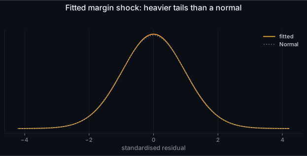
We don't predict a number, we predict a distribution for the game: summarised as a margin . The centre comes from an ensemble; the shock around it is fitted from past errors and has heavier tails than a bell curve, because basketball margins do: blowouts are more common than a normal distribution predicts.
Predicting the whole distribution is what lets us read a fair probability for the head-to-head and for a handicap at any line off one object, all mutually consistent.
The predictive distribution
For each game we predict a distribution over the match margin M. The centre μ(x) comes from an ensemble fitted on prior seasons; the shock Z around it is a standardised heavy-tailed distribution (basketball margins have fat tails: blowouts happen more often than a bell curve implies). Fitting a standardised shock keeps all the scale in σ, so σ carries the model's uncertainty for that game.
Where it can mislead. The centre adapts to where in the season a match falls rather than being one fixed relationship year-round; that choice is made on held-out per-stage testing, not assumed.
From the distribution to the prices
The head-to-head price and every handicap line are read off the same margin distribution. NBL has no draw, so with a half-point continuity correction the home win probability and the cover probability at any handicap both fall out of one object, which makes the prices mutually consistent by construction.
Where it can mislead. Consistency by construction is a strength, but it also means a mis-calibrated σ shows up in every price at once.
What the model uses
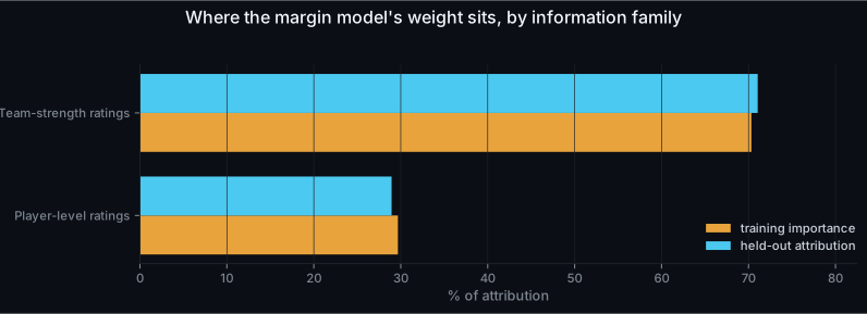
The margin model runs on two kinds of information: team-strength ratings (two independent estimators, together about two-thirds of the attribution) and player-level ratings, about a third. It is deliberately small. A liquid market already prices team strength efficiently, so beyond the ratings our edge is in the calibrated distribution and the entry timing, not in a long feature list.
We read two independent importance measures. Where they disagree on individual inputs it is because two ratings measuring nearly the same thing trade places, not because the model has found something spurious, which is why we always read both and aggregate them into families.
Split gain (tree importance)
In a tree ensemble, every time the model splits on a feature it reduces the training error by some amount. A feature's gain is the total of those reductions, shown as a share of the whole. It is a quick read on which inputs the model actually uses.
Where it can mislead. Gain is a training-set quantity and it rewards a feature simply for being split on. Two features that measure nearly the same thing will trade splits back and forth, so gain can look unstable even when the model is stable.
SHAP values
A game-theoretic way to attribute a prediction to its inputs: each feature's contribution is its average effect across every possible order in which the features could be added. We report the average size of that contribution on held-out games, not training games.
Where it can mislead. Gain and SHAP answer different questions (training-set error reduction versus held-out output attribution) and they disagree when features are collinear. That is exactly why we read both and aggregate them into families rather than trusting either alone.
Rule and roster-era changes
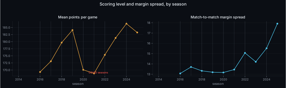
The league is not stationary. Scoring has risen materially over the sample (a continuous style shift rather than a single rule break), and the 2020–21 COVID seasons, with a Melbourne hub, cut rosters and the NBL Cup folded into the ladder, are the single most anomalous stretch on record.
So every candidate signal is screened per regime era, not just pooled, and one whose sign or size flips across a regime boundary is treated as fragile and down-weighted or dropped. The model is fitted walk-forward, so a regime change is absorbed as it happens rather than baked in from a stale full-sample fit. And we don't import structural constants from other leagues (the NBA's free-throw possession coefficient is the classic example) unless they are measured on NBL data.
Signal selection
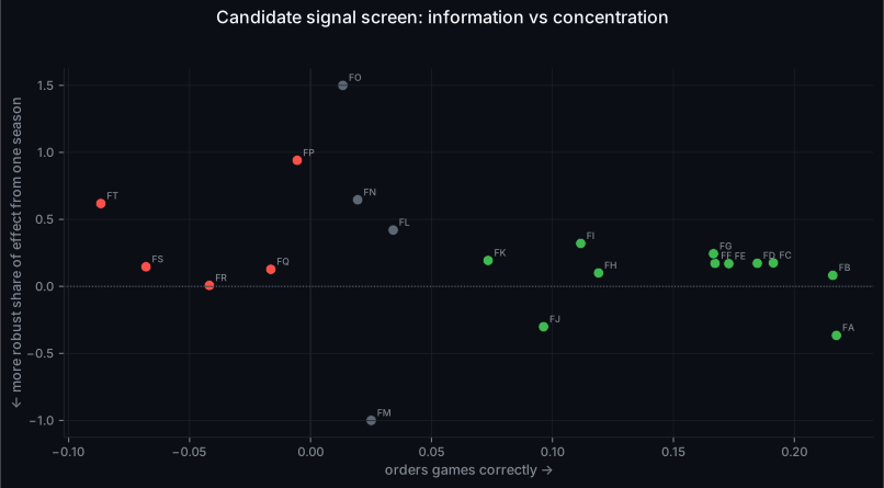
A signal is kept only if it clears two bars: a positive information coefficient with a hit rate above 50% (it orders games correctly in most rounds) and low concentration, meaning its value is not the product of one unusual season.
Most candidates cluster near zero. Genuinely useful, individually small signals are rare in this sport at this data volume, and we don't pretend otherwise. Even the kept family (team-strength ratings) hurt across the 2016 import-cap and roster-reform boundary, when every rating system was working off stale pre-reform form. That is not a reason to drop it; it is the reason the model is re-fitted walk-forward and screened per era rather than pooled.
Information coefficient
Within each betting round, does a candidate signal order the games in the right order? We take the rank correlation between the signal and the outcome, round by round, and average it. We also report the hit rate: the share of rounds where the correlation is positive.
Where it can mislead. IC measures ordering, not magnitude, so a signal can have a positive IC and still be too small to bet on. A single strong round can lift the average, which is why we pair it with the concentration check.
Concentration check
A signal can look good on a pooled average because of one unusual season. We recompute the effect with each season dropped in turn and measure how much of the apparent effect a single season is responsible for. A signal we trust has its value spread across seasons.
Where it can mislead. A high concentration is a red flag no matter how large the headline number. It is only meaningful for a signal that has a non-trivial information coefficient in the first place.
Structure and calibration
The model's centre adapts to where in the season a match falls, chosen on held-out per-stage testing rather than fixed everywhere. Adding player-level information to the margin model is a judgement call, and we label it as one: on our strict standard (a bootstrap interval excluding zero on both evaluation lenses) that addition is not proven, because its out-of-sample improvement is small and sits inside the noise. We serve it because it points the right way consistently across the walk-forward and on the 2025 holdout, and because the player signal is mechanically independent of team form.
Calibration (bias, scale, tail shape) is fitted walk-forward from past errors, and every calibration choice gets the same held-out scrutiny as any feature: several that were convincing on inner-window data did not carry to a genuinely held-out season, and were dropped.