How the model is tested
The process that checks the model: the data split, walk-forward scoring, two independent leak audits with a live positive control, and the bar a candidate has to clear before it is served.
Data split
The sample is split by time into three segments. Development seasons are where the model is built and screened; test seasons are freely inspected during selection; the final holdout (the 2025 season) was scored exactly once, after every feature, structure and calibration choice was frozen. The split exists so that choices made against the test seasons cannot contaminate the season used for the final check. The holdout number is the one we treat as the honest read.
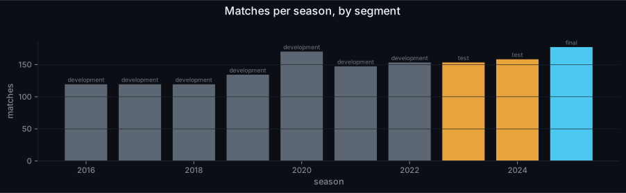
| Segment | Seasons | Role |
|---|---|---|
| Development | 2013–2022 | model built, features screened, calibration fitted, walk-forward within this window |
| Test | 2023–2024 | freely inspected during model selection; where every design decision was checked |
| Final holdout | 2025 | scored exactly once, after every feature / structure / hyperparameter choice was frozen |
| Forward | 2026– | genuinely unplayed |
Walk-forward evaluation
Every season is predicted by a model trained only on earlier seasons; the window then expands and we move on. No game is ever in its own training set, and nothing from the future of the league is available when a prediction is made.
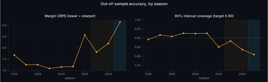
Out-of-sample accuracy is stable across the decade: margin CRPS sits in a roughly 7 to 9 band and interval coverage tracks the 90% line. Two seasons run loose and we report them rather than smooth them. 2022 was the first post-COVID "return to normal", with higher margin variance for every rating system. 2025 (the holdout) ran an unusually wide spread of margins, and the forecast was mildly over-confident against it, at about 0.81 coverage against a 0.90 target. We have since made systematic adjustments to the scale and tail calibration in anticipation of 2026 league conditions, so forward accuracy is expected to improve on this.
Walk-forward evaluation
Every season in the backtest is predicted by a model trained only on earlier seasons, then the window expands and we move on. No game is ever in its own training data, and nothing from the future of the league is available when a prediction is made. The distribution's calibration is fixed from pre-2023 data and never re-fitted forward, so the track record carries no hindsight.
Where it can mislead. Walk-forward is the honest way to score a time series, but early seasons are predicted from very little history, so the first year or two of any backtest is noisier than the rest.
CRPS: Continuous Ranked Probability Score
Our main accuracy score. It compares the whole predicted distribution F against the one number that actually happened, y. It is strictly proper: a model can only improve its CRPS by stating its real uncertainty, never by bluffing, and it collapses to plain mean absolute error when the forecast is a single number, so it reads on the same scale as points. Lower is better.
Where it can mislead. CRPS rewards a sharp, calibrated distribution, but it does not translate one-for-one into profit: a model that quietly predicts the same average distribution for every game can still score well while having nothing useful to say about which side to bet.
Leak audits
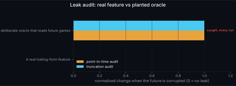
Two independent audits. The first replaces every match result on or after a cutoff date with noise and recomputes every feature for earlier matches: a feature that only uses the past is numerically unchanged. The second deletes all rows on or after the cutoff and recomputes, which catches features that quietly use a whole-sample statistic.
We keep a deliberately leaky "oracle" feature that reads future results as a positive control. Both audits flag it, every run. Every feature group in the live model passes both audits, at two different cutoff dates. Separately, we re-derived the walk-forward predictions from scratch outside the production pipeline and reproduced them exactly.
Leak audits
Two independent tests. First: replace every match result on or after a cutoff date with noise, then recompute every feature for matches before the cutoff: a feature that only uses the past is numerically unchanged. Second: delete all rows on or after the cutoff and recompute, this catches features that quietly use a whole-sample statistic. We keep a deliberately leaky "oracle" feature that reads future results as a positive control; both audits must flag it on every run.
Where it can mislead. The audits prove a feature does not peek at the future. They do not prove the feature is useful. That is what the walk-forward score and the bootstrap bar are for.
The adoption bar
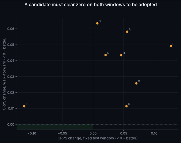
A candidate is scored two ways: on a fixed test window and on the expanding walk-forward window. To be adopted it must clear a per-match bootstrap interval that excludes zero on both at once. This is a deliberately narrow target. The two windows weight different seasons, so anything that clears both is robust to which seasons happen to land in the sample; anything that clears only one is, at our data volume, indistinguishable from noise and is not adopted.
Therefore the served model carries few moving parts, and each one has cleared the same bar. Additions that point the right way on both windows without the interval clearing zero (the player-rating group is the example) are served but labelled as unproven rather than counted as edge.
Bootstrap confidence intervals
To put an honest error bar on an average (profit per bet, a win rate, a CRPS gap) we resample the observations we have, with replacement, ten thousand times, recompute the average each time, and take the middle 95% of those values. We only call something demonstrated when this interval sits entirely on one side of zero. We lean on the bootstrap rather than a parametric error bar specifically because the NBL samples are small: a few hundred bets across roughly two hundred matches, so it makes no distributional assumptions the data can't support.
Where it can mislead. The bet rows are not fully independent (one match can be entered on several days), so we resample whole rows and always quote the match count next to the sample size. A significant t-statistic on a single fixed test set is not enough at our sample sizes.
From distribution to price
Every price is a deterministic transform of the forecast; there are no free parameters between the forecast and the quote. NBL has no draw, so with a half-point continuity correction the home-win probability is and the probability the home team covers a handicap is .
The head-to-head price and the whole handicap ladder therefore come from one distribution, from which "edge" is our fair probability minus the market's de-vigged one, expressed as expected value at the price on offer.
The predictive distribution
For each game we predict a distribution over the match margin M. The centre μ(x) comes from an ensemble fitted on prior seasons; the shock Z around it is a standardised heavy-tailed distribution (basketball margins have fat tails: blowouts happen more often than a bell curve implies). Fitting a standardised shock keeps all the scale in σ, so σ carries the model's uncertainty for that game.
Where it can mislead. The centre adapts to where in the season a match falls rather than being one fixed relationship year-round; that choice is made on held-out per-stage testing, not assumed.
From the distribution to the prices
The head-to-head price and every handicap line are read off the same margin distribution. NBL has no draw, so with a half-point continuity correction the home win probability and the cover probability at any handicap both fall out of one object, which makes the prices mutually consistent by construction.
Where it can mislead. Consistency by construction is a strength, but it also means a mis-calibrated σ shows up in every price at once.
De-vigging a two-way market
Bookmaker prices carry a margin, so the raw implied probabilities from the two sides of a market add up to more than 100%. Dividing each by that total recovers the market's implied fair probabilities. Every "market probability" on these pages is de-vigged this way, so model-versus-market comparisons are like-for-like.
Where it can mislead. Splitting the margin evenly across both sides is the simplest de-vig and the one we use; other methods exist and shift the fair line slightly, especially on lopsided prices.
Expected value and claimed edge
At our probability p for an outcome priced at decimal odds o, a one-unit bet pays o − 1 with probability p and loses 1 otherwise. We bet the side of a market with the larger expected value, and call that number the claimed edge.
Where it can mislead. Claimed edge is our estimate of value, not a realised result. In this project it turned out not to rank which bets actually win: the entry-timing section covers this.